2.5. ARRAY LIBRARIES

2.4. OPTIMIZING COMPILERS

Vector and superscalar architectures provide more performance potential than the serial scalar architecture. Vector and superscalar architectures are an evolution of this traditional architecture and include the latter as a particular case. For this reason programming tools for the architectures are mainly based on C and Fortran.

These tools include optimizing C and Fortran 77 compilers. The main specific optimization is loop vectorization. The compilers try to recognize the loops, which are in fact a sequential form of vector operations, and compile the loops in the most efficient way. For example, consider the following loop:

 for(i=0; i<64; i++)   c[i] = a[i] + b[i] ; 

This implements addition of two real vectors. Straightforward compilation of the loop leads to the target code of the form

        r0 <- 0 begin:  if(r0>=64) goto end         r1 <- a[r0]         r2 <- b[r0]         r3 <- r1 + r2         c[r0] <- r3         r0 <- r0 + SIZE_OF_TYPE         goto begin end:    continue 

where r0, r1, r2, r3 are scalar registers, a, b, c are address constants (addresses of the first element of the corresponding arrays), and SIZE_OF_TYPE is a integer constant (the size of elements of real arrays a, b, and c). The target code takes no advantage of the vector processor because it does not use vector instructions. It is also not able to load pipelined units of the superscalar processor because the instructions of the program, which could be executed in parallel by the same IEU, have conflicting operands: namely the addition instruction

r3 <- r1 + r2

writes in the same register r3 at successive iterations of the loop. In addition, in the control flow, the instructions are separated by several other instructions and hence cannot fully load the corresponding pipeline even in the absence of conflicting operands.

Thus the straightforward compilation scheme is not able to accelerate the execution of the array operation. At the same time, for the vector processor, the loop could be efficiently implemented with vector instructions of the processor by the target code of the form

v1 <- a v2 <- b v3 <- v1 + v2 c <- v3

where v1, v2, v3 are vector registers (for simplicity, we assume that the size of the vector registers is 64).

For the superscalar processor, the loop could be efficiently implemented by unrolling the loop in order to load the best possible pipelined units of the processor. For example, an optimizing compiler for the superscalar processor could generate the following target code

      r0 <- 0 begin:if(r0>=64) goto end       r1 <- a[r0]       r2 <- a[r0+SIZE_OF_TYPE]       r3 <- a[r0+2*SIZE_OF_TYPE]       r4 <- a[r0+3*SIZE_OF_TYPE]       r5 <- a[r0+4*SIZE_OF_TYPE]       r6 <- a[r0+5*SIZE_OF_TYPE]       r7 <- a[r0+6*SIZE_OF_TYPE]       r8 <- a[r0+7*SIZE_OF_TYPE]       r9 <- b[r0]       r10 <- b[r0+SIZE_OF_TYPE]       r11 <- b[r0+2*SIZE_OF_TYPE]       r12 <- b[r0+3*SIZE_OF_TYPE]       r13 <- b[r0+4*SIZE_OF_TYPE]       r14 <- b[r0+5*SIZE_OF_TYPE]       r15 <- b[r0+6*SIZE_OF_TYPE]       r16 <- b[r0+7*SIZE_OF_TYPE]       r17 <- r1 + r9       r18 <- r2 + r10       r19 <- r3 + r11       r20 <- r4 + r12       r21 <- r5 + r13       r22 <- r6 + r14       r23 <- r7 + r15       r24 <- r8 + r16       c[r0] <- r17       c[r0+SIZE_OF_TYPE] <- r18       c[r0+2*SIZE_OF_TYPE] <- r19       c[r0+3*SIZE_OF_TYPE] <- r20       c[r0+4*SIZE_OF_TYPE] <- r21       c[r0+5*SIZE_OF_TYPE] <- r22       c[r0+6*SIZE_OF_TYPE] <- r24       c[r0+7*SIZE_OF_TYPE] <- r24       r0 <- r0 + 8*SIZE_OF_TYPE       goto begin end:  continue 

This code is able to load the pipeline unit executing reading from memory into registers, the pipeline unit executing addition of two registers, and the pipeline unit executing writing into memory from registers. Some compilers for superscalar processors perform a more general loop parallelization—the loop pipelining, including loop vectorization as a particular case.

The most difficult problem to be solved by the optimizing compilers is recognition of the loops, whether parallelized or vectorized. The solution is based on the analysis of data dependencies in loops. In general, there are three classes of data dependence between statements in sequential programs that must be determined for the statements to be executed in parallel: flow dependence (or true dependence), anti-dependence, and output dependence. True dependence exists between a statement of the form

x = a + b ;

and a statement of the form

c = x + d ;

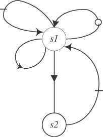
In other words, true dependence exists between statement s1, which writes in some variable, and statement s2, which follows (in control flow) statement s1 and uses this variable. In graphical form this dependence is depicted as follows:

Anti-dependence exists between a statement of the form

a = x + b ;

and a statement of the form

x = c + d ;

In other words, anti-dependence exists between statement s1, which uses some variable, and statement s2, which follows (in control flow) statement s1 and writes in this variable. In graphical form this dependence is depicted as follows:

Output dependence exists between a statement of the form

x = a + b ; 

and a statement of the form

x = c + d ;

In other words, output dependence exists between statement s1, which writes in some variable, and statement s2, which follows (in control flow) statement s1 and also writes in this variable. In graphical form this dependence is depicted as follows:

To decide if a loop can be parallelized or vectorized, its dependence graph should be built. The dependence graph for the loop is built as a summary of the dependence graph for the result of the unrolling of the loop. For example, the full “unrolled” dependence graph for the loop

 for(i=0; i<n; i++) {   c = a[i] + b[i] ; /* statement s1 */   d[i] = c + e[i] ; /* statement s2 */ }

looks as follows:

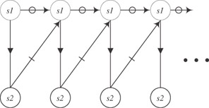
This potentially infinite graph is summarized in the form of the finite graph

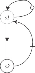
Usually during the summarizing some information is lost. For example, the loop

 for(i=0; i<n; i++) {   c[i] = a[i] + b ;      /* statement s1 */   d[i] = c[i] + e[i] ;   /* statement s2 */ }

has the same dependence graph of the form

as the loop

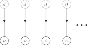
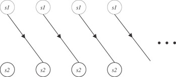
 for(i=0; i<n; i++) {   c[i+1] = a[i] + b ;      /* statement s1 */   d[i] = c[i] + e[i] ;     /* statement s2 */ }

However, their unrolled dependence graphs are different. The unrolled dependence graph for the first loop is

The unrolled dependence graph for the second loop is

The importance of the dependence analysis of loops is explained by a simple fact: A loop whose dependence graph is cycle-free can be parallelized or vectorized. The reason is that if there are no cycles in the dependence graph, then there will be no races in parallel execution of the same statement from different iterations of the loop.

Note that the presence of cycles in the dependence graph does not mean that the loop cannot be vectorized or parallelized. The point is that some cycles in the dependence graph can be eliminated by using elementary transformations. For example, the loop

 for(i=0; i<n; i++) {   c = a[i] + b[i] ; /* statement s1 */   d[i] = c + e[i] ; /* statement s2 */ }

whose dependence graph is

can be transformed into the loop

 for(i=0; i<n; i++) {       cc[i] = a[i] + b[i] ; /* statement s1 */       d[i] = cc[i] + e[i] ; /* statement s2 */ } c = cc[n-1] ;

whose dependence graph has no cycle:

The transformation is known as scalar expansion.

Another transformation that eliminates cycles in dependence graphs is induction variable recognition. This transformation is used to transform the loop

 for(i=0; i<n; i++) {   a = a + b ;       /* statement s1 */   c[i] = c[i] + a ; /* statement s2 */ }

whose dependence graph is

into the loop

 for(i=0; i<n; i++) {   d[i] = a + b*i ;       /* statement s1 */   c[i] = c[i] + d[i] ;   /* statement s2 */ }

whose dependence graph has no cycle:

So far building the dependence graph for a loop has proved not so difficult. This is explained by simplicity of subscript expressions in the loops we have analyzed. But the problem of testing dependences in loops can be very complex and expensive. To see this, let us define some dependences in loops in a more general and formal way. For a loop of the form

 for(i=0; i<n; i++) {   c[f(i)] = a[i] + b[i] ; /* statement s1 */   d[i] = c[g(i)] + e[i] ; /* statement s2 */ }

a true dependence between statement s1 and statement s2 exists if and only if Ǝi, j Є [0, n - 1]:i ≤ j & f(i) = g(j), and an anti-dependence between statement s2 and statement s1 exists if and only if Ǝi, j Є [0, n - 1]:i > j & f(i) = g(j). For a loop of the form

optimizing compilers

 for(i=0; i<n; i++) {   c[i] = a[g(i)] + b[i] ; /* statement s1 */   a[f(i)] = d[i] + e[i] ; /* statement s2 */ }

a true dependence between statement s2 and statement s1 exists if and only if Ǝi, j Є [0, n - 1]:i < j & f(i) = g(j).

The problem of testing these conditions can be NP-complete and hence very expensive. Therefore the practical tests used in optimizing compilers usually assume that subscript expressions are simple: namely that f(i) = a₁ X i + a₀ and g(i) = b₁ X i + b₀. Then f(i) = g(j) if and only if a₁ X i - b₁ X j = b₀ - a₀. The approach that has traditionally been used is to try to break a dependence, that is, to try to prove that the dependence does not exist.

One simple practical test is the GCD test. The test breaks the dependence if there is no integer solution to the equation a₁ X i - b₁ X j = b₀ - a₀, ignoring the loop limits. A solution to the equation a₁ X i - b₁ X j = b₀ - a₀ exists if and only if the greatest common divisor (GCD) of a₁ and b₁ divides b₀ - a₀. The test is conservative. That is, it may not break a dependence that does not exist. Indeed, the equation could have solutions outside the iteration space only. A conservative test can guarantee the absence of the dependence but may not guarantee its presence. In other words, if the test fails to prove the absence of the dependence, it does not necessarily mean that the dependence is present. Practical tests are usually conservative.

A more accurate test taking into account the loop limits is Banerjee’s test. It proceeds by finding an upper bound U, and a lower bound L of a₁ X i - b₁ X j under the constraints that 0 ≤ i < n and 0 ≤ j < n. If either L > b₀ - a₀ or U < b₀ - a₀, then the functions do not intersect, and therefore there is no dependence. For example, consider the loop

 for(i=0; i<10; i++) {   c[i+10] = a[i] + b[i] ;    /* statement s1 */   d[i] = c[i] + e[i] ;       /* statement s2 */ }

The GCD test will not break the dependence between statements s1 and s2 because there is a solution to the equation a₁ X i - b₁ X j = b₀ - a₀ or i - j = -10. However, the lower bound of a₁ X i - b₁ X j = i - j is -9, which is greater than b₀ - a₀, and therefore the dependence would be broken by the Banerjee test.

The same procedure for the loop

 for(i=0; i<10; i++) {   c[i+9] = a[i] + b[i] ;     /* statement s1 */   d[i] = c[i] + e[i] ;       /* statement s2 */ } 

will not break the dependence because the lower bound of a₁ X i - b₁ X j = i - j is -9, which is not greater than b₀ - a₀ = -9. In this case the accuracy of dependence analysis can be increased by testing possible dependences between statements s1 and s2 separately. Namely, to test the anti-dependence between statements s2 and s1, the restriction i > j should be added to the loop limits when computing the upper and lower bounds. Then the lower bound of a₁ X i - b₁ X j = i - j is 1, which is greater than b₀ - a₀ = -9 and therefore the anti-dependence is broken by the test. To test the true dependence between statements s1 and s2, the restriction i ≤ j should be added to the loop limits when computing the upper and lower bounds of a₁ X i - b₁ X j. Then the lower bound of a₁ X i - b₁ X j = i - j is -9, which is not greater than b₀ - a₀, and therefore the true dependence is not broken. This more accurate analysis allows us to conclude that even though there may exist a true dependence between statements s1 and s2, other dependences between the statements do not exist, and therefore the dependence graph for the loop is cycle-free, which means that the loop can be parallelized or vectorized.

This more accurate test can be formulated in terms of directions. Note that testing all types of dependence between statements s1 and s2 reduces to computing an upper bound U, and a lower bound L of a₁ X i - b₁ X j under the constraints that 0 ≤ i < n and 0 ≤ j < n. Testing different types of dependence only differs in the direction of the dependence in the iteration space: at the same iteration (i = j), between different iterations in forward direction (i < j), and between different iterations in backward direction (i > j).

In general, given a loop nest

 for(i1=...)   for(i2=...)     ...       for(ik=...){   a[f(i1,i2,...,ik)] =…      /* statement s1 */   ... = a[g(i1,i2,...,ik)] ; /* statement s2 */ }

the complete Banerjee test would check dependencies for each possible direction. Namely, for all valid direction vectors (ψ₁, ψ₂,…, ψ_k) with each ψ_i is either <, >, or =, the test tries to show that there is no solution to the equation

within the loop limits, with the restrictions

These restrictions are taken into account when computing the upper and lower bounds (in the complete test, there is a pair of lower and upper bounds for each loop index).

There are at least three reasons why Banerjee’s test is conservative. First, it only checks that there is a real-valued solution to the equation. The solution does not have to be integer. Therefore failure to break the dependence does not imply that the dependence exists.

Second, for multiple subscript arrays, each subscript equation is tested separately. A dependence will be assumed if there is a solution for each separate equation. This is conservative because the system of equations may not have a solution even though each equation has a solution.

Third, it is assumed that the loop limits and the coefficients are known constants. This assumption can be relaxed as the test will still work if loop limit are set to infinity. However, dependence is assumed if one of the coefficients is not known.

Apart from the GCD test and the Banerjee inequalities test, there are some other practical dependence tests such as the Rice partition-based test, the Stanford cascade test, and the Maryland Omega test.

Different optimizing compilers use different algorithms to recognize parallelizable loops. Each compiler has its own class of parallelizable loops, and the classes for different compilers can differ significantly. Therefore, although optimizing C and Fortran 77 compilers are able to generate efficient codes for vector and superscalar architectures, the writing of the corresponding source codes is often not trivial. The programmer must know the particular compiler very well to use exactly those forms of parallelizable loops that are recognized by the compiler. As a result some applications that run efficiently on one vector or superscalar processor, due to their careful tuning to the corresponding compiler, may run much slower on other vector and superscalar processors of the same potential performance. Although there are some simple classes of parallelizable loops that are recognized by any normal optimizing compiler for vector or superscalar processor, these classes are quite restricted and do not include many real-life loop patterns.

Our analysis of optimizing C and Fortran 77 compilers for vector and superscalar processors can be summarized as follows:

• Like those for the serial architecture, the compilers support modular, portable, and reliable programming.

• The compilers support efficient programming but for rather restricted class of applications; the efficient programming is quite demanding for the programmer and often leads to such source code that is difficult to read and understand.

• The support for portable efficiency provided by the compilers is limited to some very simple classes of application.