Performance by Design. Computer Capacity Planning by Example 

11.7 Approximation Results

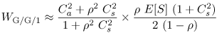
M/G/1 results cannot be used when the interarrival time distribution is not exponentially distributed. However, the approximation

Equation 11.7.25

where C _a is the coefficient of variation of the interarrival time is useful [2].

This approximation is exact for M/G/1. To verify this, note that in the M/G/1 case, C _a = 1 since interarrival times are exponentially distributed. Thus, the first term of the equation becomes one and the second term is the M/G/1 result of Eq. (11.4.14). The approximation of Eq. (11.7.25) is good for G/M/1 queues. It is "fair" for G/G/1 queues and improves as r increases .

Example 11.8.

Measurements taken from a storage device used by a database server indicate that I/O requests arrive at an average rate of 80 requests /sec. The standard deviation of the interarrival time is measured as 0.025 sec. The average I/O time is measured as 0.009 sec with a standard deviation of 0.003 sec. What is the approximate waiting time of an I/O request at the storage device?

The average interarrival time is the inverse of the average arrival rate. Thus, = 1/80 = 0.0125 sec. The coefficient of variation of the interarrival time is C _a = s _a = 0.025/0.0125 = 2. The utilization of the storage device is r = l x E [ S ] = 80 x 0.009 = 0.72. The coefficient of variation of the service time is C _s = s _s / E [ S ] = 0.003/0.009 = 1/3. Equation (11.7.25) can be used to approximate the average waiting time at the storage device:

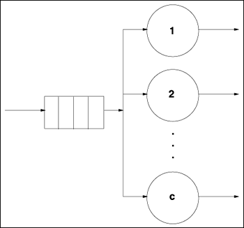
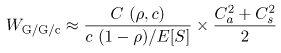
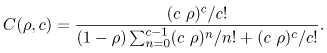
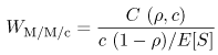
Equation 11.7.26

If C _a were equal to one, the average waiting time would be 0.0129 sec according to the M/G/1 result (i.e., Eq. (11.4.14)). This example further demonstrates the rule of thumb that increased variability (as indicated by the coefficient of variation) hurts performance).

Consider now the queue of Fig. 11.4 which has c identical servers and a single waiting line. This is known as the G/G/c queue and its utilization is

Equation 11.7.27

The exact solution for G/G/c is not known but its average waiting time can be approximated by

Equation 11.7.28

where

Equation 11.7.29

This equation is Erlang's C formula [2]. The error in the approximation of Eq. (11.7.28) increases with C _a and with C _s . In the case of an M/M/c system (i.e., exponentially distributed interarrival times and exponentially distributed service times), the approximation of Eq. (11.7.28) is an exact solution and becomes

Equation 11.7.30

because C _a = 1 and C _s = 1 for this case.

Example 11.9.

A computer system receives requests that require an average of 2 seconds of service time. The coefficient of variation of the service time is 0.5 and the coefficient of variation of the interarrival time is 0.8. What is the minimum number of processors that should be used to keep the average response time below 2.5 seconds when the utilization of the system is 80%.

The question can be answered by using the G/G/c approximation of Eq. (11.7.28). The required parameters are: r = 0.80, C _a = 0.8, C _s = 0.5, and E [ S ] = 2 sec. The number of processors, c , is varied from 1 to 8. The results are presented in Table 11.3, which shows that at least 5 processors are needed.

Table 11.3. Response Time (sec) vs. No. Processors